Test if gvxrPython3 is well installed
To check that gvxrPython3 (SimpleGVXR’s Python3 wrapper) is well compiled and installed, try the following command in the prompt:
$ python3 -c 'import gvxrPython3 as gvxr; print(gvxr.getMajorVersionOfSimpleGVXR())'
If you get the following error, it’s because it is not installed properly or it cannot find gvxrPython3, refer to the instll guide in Section 5
Traceback (most recent call last):
  File "<string>", line 1, in <module>
ModuleNotFoundError: No module named 'gvxrPython3'
If you see the output message is 1, then all is fine and you can proceed.
Simulating an X-ray projection from a STL file
$ wget https://sourceforge.net/p/gvirtualxray/code/HEAD/tree/trunk/SimpleGVXR-examples/WelshDragon/welsh-dragon-small.stl
or use the one provided in this directory.
- Launch the Python interpreter and load the packages
#!/usr/bin/env python3

try:
    import matplotlib
    matplotlib.use("TkAgg")

    import matplotlib.pyplot as plt
    import matplotlib.image as mpimg
    from matplotlib.colors import LogNorm
    from matplotlib.colors import PowerNorm
    use_matplotlib = True;
except ImportError:
    print("Matplotlib is not installed. Try to install it if you want to display and plot data.")
    use_matplotlib = False;

import gvxrPython3 as gvxr
- If Matplotlib is available, create the subplot first
if use_matplotlib:
    plt.subplot(131)
gvxr.createWindow();
gvxr.setWindowSize(512, 512);
gvxr.setSourcePosition(-40.0,  0.0, 0.0, "cm");
gvxr.usePointSource();
#gvxr.useParallelBeam();
gvxr.setMonoChromatic(0.08, "MeV", 1000);
gvxr.setDetectorPosition(10.0, 0.0, 0.0, "cm");
gvxr.setDetectorUpVector(0, 0, -1);
gvxr.setDetectorNumberOfPixels(640, 320);
gvxr.setDetectorPixelSize(0.5, 0.5, "mm");
gvxr.loadSceneGraph("welsh-dragon-small.stl", "mm");

# Get the label
label = gvxr.getChildLabel('root', 0);

# Move label to the centre
gvxr.moveToCentre(label);

# Move the mesh to the center
gvxr.moveToCenter(label);

# Set the material properties
gvxr.setHU(label, 1000);
- Compute an X-ray image and save it
x_ray_image = gvxr.computeXRayImage();

gvxr.saveLastXRayImage("my_beautiful_dragon.mhd");
gvxr.saveLastXRayImage("my_beautiful_dragon.mha");
gvxr.saveLastXRayImage("my_beautiful_dragon.txt");
- Display the image with Matplotlib
if use_matplotlib:
    plt.imshow(x_ray_image, cmap="gray");
    plt.colorbar(orientation='horizontal');
    plt.title("Using a linear colour scale");

    plt.subplot(132)
    plt.imshow(x_ray_image, norm=LogNorm(), cmap="gray");
    plt.colorbar(orientation='horizontal');
    plt.title("Using a log colour scale");

    plt.subplot(133)
    plt.imshow(x_ray_image, norm=PowerNorm(gamma=1./2.), cmap="gray");
    plt.colorbar(orientation='horizontal');
    plt.title("Using a Power-law colour scale");

    plt.show();
- Interactive visualisation of the 3D environment
# Display the 3D scene (no event loop)
# Run an interactive loop
# (can rotate the 3D scene and zoom-in)
# Keys are:
# Q/Escape: to quit the event loop (does not close the window)
# B: display/hide the X-ray beam
# W: display the polygon meshes in solid or wireframe
# N: display the X-ray image in negative or positive
# H: display/hide the X-ray detector
gvxr.renderLoop();
or execute xray_proj_from_INP.py.
Simulating an X-ray projection from a INP file
- Launch the Python interpreter and load the packages
#!/usr/bin/env python3

import os, copy
import numpy as np
dir_path = os.path.dirname(os.path.realpath(__file__))

# Use Matplotlib
try:
    import matplotlib
    matplotlib.use("TkAgg")

    import matplotlib.pyplot as plt
    import matplotlib.image as mpimg
    from matplotlib.colors import LogNorm
    from matplotlib.colors import PowerNorm
    use_matplotlib = True;
except ImportError:
    print("Matplotlib is not installed. Try to install it if you want to display and plot data.")
    use_matplotlib = False;

import gvxrPython3 as gvxr
import inp2stl
- If Matplotlib is available, create the subplot first
# Create the subplot first
# If called later, it crashes on my Macbook Pro
if use_matplotlib:
    plt.subplot(131)
print("Create an OpenGL context")
gvxr.createWindow();
gvxr.setWindowSize(512, 512);
gvxr.setSourcePosition(-40.0,  0.0, 0.0, "cm");
#gvxr.usePointSource();
gvxr.useParallelBeam();
gvxr.setMonoChromatic(0.08, "MeV", 1000);
gvxr.setDetectorPosition(40.0, 0.0, 0.0, "cm");
gvxr.setDetectorUpVector(0, 0, -1);
gvxr.setDetectorNumberOfPixels(640, 320);
gvxr.setDetectorPixelSize(0.5, 0.5, "mm");
- Load the data from the INP file
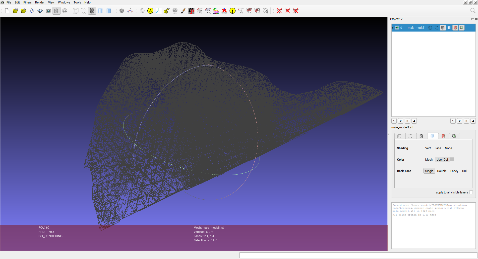
vertex_set, triangle_index_set, material_set = inp2stl.readInpFile('male_model.inp', True);
#inp2stl.writeStlFile("male_model.stl", vertex_set, triangle_index_set[0]);
min_corner = None;
max_corner = None;

vertex_set = np.array(vertex_set).astype(np.float32);

for triangle in triangle_index_set[0]:
    for vertex_id in triangle:


        if isinstance(min_corner, NoneType):
            min_corner = copy.deepcopy(vertex_set[vertex_id]);
        else:
            min_corner[0] = min(min_corner[0], vertex_set[vertex_id][0]);
            min_corner[1] = min(min_corner[1], vertex_set[vertex_id][1]);
            min_corner[2] = min(min_corner[2], vertex_set[vertex_id][2]);

        if isinstance(max_corner, NoneType):
            max_corner = copy.deepcopy(vertex_set[vertex_id]);
        else:
            max_corner[0] = max(max_corner[0], vertex_set[vertex_id][0]);
            max_corner[1] = max(max_corner[1], vertex_set[vertex_id][1]);
            max_corner[2] = max(max_corner[2], vertex_set[vertex_id][2]);

# Compute the bounding box
bbox_range = [max_corner[0] - min_corner[0],
    max_corner[1] - min_corner[1],
    max_corner[2] - min_corner[2]];

# print("X Range:", min_corner[0], "to", max_corner[0], "(delta:", bbox_range[0], ")")
# print("Y Range:", min_corner[1], "to", max_corner[1], "(delta:", bbox_range[1], ")")
# print("Z Range:", min_corner[2], "to", max_corner[2], "(delta:", bbox_range[2], ")")
for vertex_id in range(len(vertex_set)):
    vertex_set[vertex_id][0] -= min_corner[0] + bbox_range[0] / 2.0;
    vertex_set[vertex_id][1] -= min_corner[1] + bbox_range[1] / 2.0;
    vertex_set[vertex_id][2] -= min_corner[2] + bbox_range[2] / 2.0;
- Load the mesh ion the GPU memory
gvxr.makeTriangularMesh("male_model",
        np.array(vertex_set).astype(np.float32).flatten(),
        np.array(triangle_index_set).astype(np.int32).flatten(),
        "m");
- The model is made of Hydrogen
gvxr.setElement("male_model", "H");
- Add the mesh to the simulation
gvxr.addPolygonMeshAsInnerSurface("male_model");
- Compute an X-ray image and save it
x_ray_image = gvxr.computeXRayImage();

gvxr.saveLastXRayImage("male_model.mhd");
gvxr.saveLastXRayImage("male_model.mha");
gvxr.saveLastXRayImage("male_model.txt");
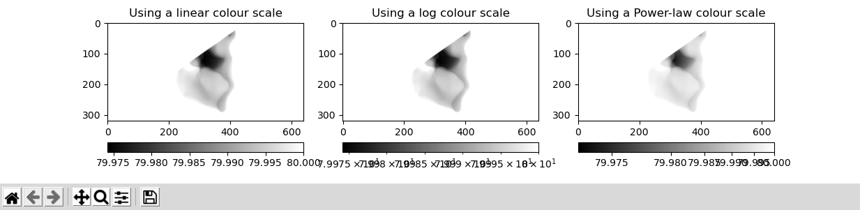
- Display the image with Matplotlib
if use_matplotlib:
    plt.imshow(x_ray_image, cmap="gray");
    plt.colorbar(orientation='horizontal');
    plt.title("Using a linear colour scale");

    plt.subplot(132)
    plt.imshow(x_ray_image, norm=LogNorm(), cmap="gray");
    plt.colorbar(orientation='horizontal');
    plt.title("Using a log colour scale");

    plt.subplot(133)
    plt.imshow(x_ray_image, norm=PowerNorm(gamma=1./2.), cmap="gray");
    plt.colorbar(orientation='horizontal');
    plt.title("Using a Power-law colour scale");

    plt.show();
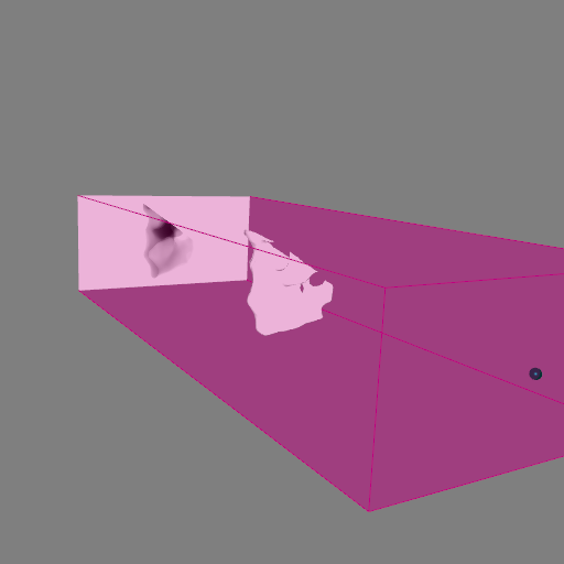
- Interactive visualisation of the 3D environment
# Display the 3D scene (no event loop)
# Run an interactive loop
# (can rotate the 3D scene and zoom-in)
# Keys are:
# Q/Escape: to quit the event loop (does not close the window)
# B: display/hide the X-ray beam
# W: display the polygon meshes in solid or wireframe
# N: display the X-ray image in negative or positive
# H: display/hide the X-ray detector
gvxr.renderLoop();
or execute xray_proj_from_INP.py.
CT acquisition
It is basically the same as previously, but with a for loop to rotate the scanned object.
projections = [];
for i in range(180):
    # Compute an X-ray image and add it to the list of projections
    projections.append(gvxr.computeXRayImage());

    # Save the X-ray image
    gvxr.saveLastXRayImage("male_model_projection_" + '{0:03d}'.format(i) + ".dcm");

    # Update the 3D visualisation
    gvxr.displayScene();

    # Rotate the model by 1 degree
    gvxr.rotateNode("male_model", 1, 0, 0, -1);
or execute ct_acquisition.py.
CT reconstruction using tomopy
It is fairly similar to the previous program, but
- I added a few extract packages:
import math # for pi
import tomopy # for tomography reconstruction
import SimpleITK as sitk # for saving the CT volume
- Pixel spacing is now in a variable for future use
spacing_in_mm = 0.5;
gvxr.setDetectorPixelSize(spacing_in_mm, spacing_in_mm, "mm");
- We store the rotation angles in radian in an array
projections = [];
theta = [];

for i in range(360):
    # Compute an X-ray image and add it to the list of projections
    projections.append(gvxr.computeXRayImage());

    # Update the 3D visualisation
    gvxr.displayScene();

    # Rotate the model by 1 degree
    gvxr.rotateNode("male_model", 0.5, 0, 0, -1);

    # Add the corresponding angle
    theta.append(i * 0.5 * math.pi / 180);
- Convert the projections as a Numpy array
projections = np.array(projections);
- Retrieve the total energy
energy_bins = gvxr.getEnergyBins("MeV");
photon_count_per_bin = gvxr.getPhotonCountEnergyBins();

total_energy = 0.0;
for energy, count in zip(energy_bins, photon_count_per_bin):
    total_energy += energy * count;
- Perform the flat-field correction of raw data
dark = np.zeros(projections.shape);
flat = np.ones(projections.shape) * total_energy;

projections = tomopy.normalize(projections, flat, dark)
- Calculate -log(projections) to linearize transmission tomography data
projections = tomopy.minus_log(projections)
rot_center = int(projections.shape[2]/2);
- Perform the reconstruction
recon = tomopy.recon(projections, theta, center=rot_center, algorithm='gridrec', sinogram_order=False)
- Plot the slice in the middle of the volume
plt.imshow(recon[int(projections.shape[1]/2), :, :])
plt.show()
volume = sitk.GetImageFromArray(recon);
volume.SetSpacing([spacing_in_mm, spacing_in_mm, spacing_in_mm]);
sitk.WriteImage(volume, 'recon.mhd');
or execute ct_reconstruction.py.
CT reconstruction using skimage
It is fairly similar to the previous program again, but using skimage rather than tomopy.
import math # for pi
from skimage.transform import iradon, iradon_sart # for tomography reconstruction
import SimpleITK as sitk # for saving the CT volume
- This time the model is made of silicon carbide rather than hydrogen
gvxr.setCompound("male_model", "SiC");

gvxr.setDensity("male_model",
                3.2,
                "g/cm3");
- theta stores the rotation angles in degrees rather than radians.
theta.append(i * rotation_angle);
- Transformations from raw X-ray proejctions to sinograms are performed manually
# Perform the flat-field correction of raw data
dark = np.zeros(projections.shape);
flat = np.ones(projections.shape) * total_energy;
projections = (projections - dark) / (flat - dark);

# Calculate  -log(projections)  to linearize transmission tomography data
projections = -np.log(projections)

# Resample as a sinogram stack
sinograms = np.swapaxes(projections, 0, 1);
- The CT reconstruction is performed slice by slice
# Perform the reconstruction
# Process slice by slice
recon_fbp = [];
recon_sart = [];
slice_id = 0;
for sinogram in sinograms:
    slice_id+=1;
    print("Reconstruct slice #", slice_id, "/", number_of_angles);
    recon_fbp.append(iradon(sinogram.T, theta=theta, circle=True));

    # Two iterations of SART
    # recon_sart.append(iradon_sart(sinogram.T, theta=theta));
    # recon_sart[-1] = iradon_sart(sinogram.T, theta=theta, image=recon_sart[-1]);

recon_fbp = np.array(recon_fbp);
skimage‘s CT reconstruction is much slower than tomopy’s’, but it’s readily available for any Python distribution…
or execute ct_reconstruction.py.